By Wu Peng, Senior Process Instrumentation Engineer · Last reviewed August 11, 2026
A differential pressure flow calculation converts the pressure drop across a flow element into a flow rate using the square-root law: Q = K · √ΔP. Flow rises with the square root of the differential pressure, so doubling the DP raises flow by about 41 percent, and it takes four times the DP to double the flow. The constant K is fixed by the element geometry and the fluid, and the complete equation behind it is the ISO 5167 orifice equation worked through below.
That one line hides most of the calculation mistakes we see in the field: coefficients borrowed from a different form of the equation, the square root taken twice, density left at standard conditions, and milliamp signals read in the wrong mode.
This guide defines every term in the working equation, runs three worked examples with real numbers, covers the gas and steam corrections, and closes with the errors that most often put a wrong flow number on the display. The scope is pipeline flow measurement; tank-drain and nozzle-discharge formulas are a different subject.
Contents
- The working equation
- Three coefficient forms
- Rescaling with ratios
- From milliamps to flow
- One extraction only
- Gas and steam
- Sizing the element
- Common calculation errors
- Calculators and instruments
- FAQ
- Request a quote
The working equation
ISO 5167 writes the mass flow through an orifice plate, nozzle, or venturi in one standardized form. The same structure, with different coefficient values, covers every element in the differential pressure group.
qm = [C / √(1 − β⁴)] · ε · (π/4) d² · √(2 Δp · ρ₁)
Divide by density to get volumetric flow: Q = qm / ρ₁. Every symbol has a specific meaning, and two of them, the approach factor and the density, are where most hand calculations go wrong.
| Symbol | Quantity | Notes |
|---|---|---|
| C | Discharge coefficient | About 0.60 to 0.61 for a sharp-edged orifice (Reader-Harris/Gallagher equation); 0.984 to 0.995 for a classical venturi per ISO 5167-4 |
| β | Diameter ratio d/D | Bore over pipe ID; standard orifice range 0.10 to 0.75 |
| 1/√(1 − β⁴) | Velocity-of-approach factor E | 1.072 at β = 0.6, 1.147 at β = 0.7; dropping it makes the computed flow read low |
| ε | Expansibility factor | Exactly 1 for liquids; below 1 for gases and steam (next sections) |
| d | Bore diameter (m) | The bore, not the pipe; area term is (π/4)d² |
| Δp | Differential pressure (Pa) | Across the tappings, converted to pascals before entering the radical |
| ρ₁ | Upstream density (kg/m³) | At flowing pressure and temperature, never at standard conditions |
Form per ISO 5167; coefficient values are representative, and final numbers belong on the element calculation sheet.
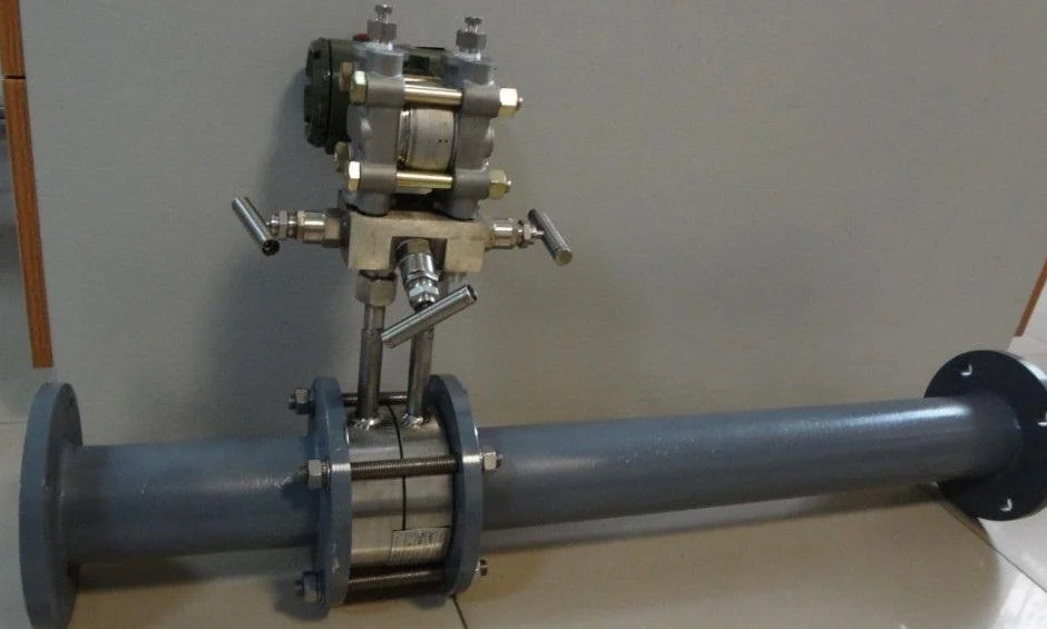
Everything in the equation except Δp is fixed once the element is built, which is why the whole expression collapses to Q = K · √ΔP in daily use. For a fully worked sizing example on water, with the beta ratio and coefficient chosen step by step, see our flow rate and pressure relationship guide.
Three coefficient forms
Published references write the same physics three ways, and the coefficients are not interchangeable between them. Before plugging in numbers, identify which form your source uses.
| Form | Equation | What the coefficient contains |
|---|---|---|
| Standards form | qm = C · E · ε · (π/4)d² · √(2Δpρ₁) | C is the discharge coefficient alone; the approach factor and the 2 are written out |
| K form | Q = K · √ΔP, or W = K · √(Δpρ) | K bundles C, the approach factor, the bore area, the factor 2, and the unit conversions; it comes from the element calculation sheet |
| Ratio form | Q₂/Q₁ = √(ΔP₂/ΔP₁) | No coefficient at all; geometry and density cancel between the two states |
One trap accounts for most coefficient mistakes. Some sources write Q = C·A·√(2ΔP/ρ) and others write Q = C·A·√(ΔP/ρ), both calling the constant a discharge coefficient. The second version has silently absorbed the √2 into its C, so the two coefficient values differ by 41 percent.
Neither equation is wrong inside its own definition; carrying a coefficient from one into the other is. Take coefficient values only from the source that defines the equation they belong to.
Rescaling with ratios
When the element already has a documented operating point, the ratio form answers most day-to-day questions without touching a single coefficient. Suppose the calculation sheet for an orifice run states 40 m³/h at 16 kPa, and the transmitter currently reads 9 kPa.
Q₂ = Q₁ · √(ΔP₂ / ΔP₁)
Q₂ = 40 · √(9 / 16) = 40 · 0.75 = 30 m³/h
The ratio form holds only while everything except the flow stays put: same element, same fluid, same density. If line pressure or temperature has moved the density since the reference point was documented, correct for that first (see the gas and steam section). And if your reading arrives as milliamps rather than kilopascals, one more question comes before any arithmetic.
From milliamps to flow
A DP transmitter on flow service sends its 4-20 mA signal in one of two modes, and the same milliamp value means two different flows. Take a transmitter ranged 0 to 40 kPa on an element sized for 60 m³/h at full DP, currently outputting 16 mA, which is 75 percent of signal span.
Linear mode: ΔP = 0.75 · 40 = 30 kPa, so Q = 60 · √(30/40) = 60 · 0.866 = 52.0 m³/h
Square-root mode: the transmitter has already extracted, so 16 mA is 75 percent of flow = 45.0 m³/h
Same signal, 7 m³/h apart. In linear mode the current follows DP and the receiving system must take the square root; in square-root mode the transmitter takes it internally and the current follows flow. Confirm which mode is configured before trusting either number: it is set in the transmitter configuration, and there are numeric signatures that reveal it from the signal itself, covered in our linear to square root conversion calculator. Range changes and trims that alter this scaling belong to transmitter calibration, not to the flow equation.
One extraction only
The square root must be applied exactly once, in exactly one device: the transmitter, the DCS input block, or the flow computer. Both failure directions produce numbers that look plausible on a display.
Extract twice and midrange readings run high. At a true flow of 50 percent, the DP sits at 25 percent of span; the first extraction correctly reports 50 percent, and a second extraction turns that into √0.50 = 70.7 percent. The display reads 41 percent above the true flow.
Skip the extraction entirely and the display follows DP instead of flow: the same true 50 percent flow shows as 25 percent. A written plant standard naming the one device that extracts is cheaper than either error.
Order matters as much as count. Density compensation belongs under the radical, applied to the Δp · ρ product before the square root is taken. Compensating a signal that has already been extracted applies the correction with the wrong weight.
Gas and steam
On liquids the density is stable enough that a fixed K carries the calculation. On gases and steam two corrections enter: the expansibility factor, and density evaluated at flowing conditions.
The expansibility factor accounts for the gas expanding as it accelerates through the bore. For orifice plates ISO 5167-2 gives:
ε = 1 − (0.351 + 0.256β⁴ + 0.93β⁸) · [1 − (p₂/p₁)1/κ]
where κ is the isentropic exponent, valid while p₂/p₁ stays at or above 0.75. On a 10 bar absolute gas line with 25 kPa of DP and β = 0.6, ε works out to about 0.992: a correction under 1 percent, small enough that it often gets skipped, and large enough to matter in custody transfer.
Density is the larger effect. A flow computer configured for saturated steam at 9.0 bar absolute uses 4.655 kg/m³ from the steam tables. Let the header slip to 8.0 bar absolute and the real density is 4.162 kg/m³; a fixed-density calculation then reads high by √(4.655/4.162) = 1.058, a 5.8 percent mass flow error from a one bar swing. Live pressure and temperature compensation removes it, which is why compensated metering is standard on steam flow meters.
The extreme version of the same mistake is using standard density on a pressurized gas: at 11 bar absolute the gas is about 11 times denser than at atmospheric, and plugging the standard value into √(Δpρ) makes the mass flow answer low by a factor of √11, about 3.3.
To run a gas calculation at all, five inputs are required: absolute static pressure at the upstream tapping, flowing temperature, the gas composition (or at minimum its specific gravity with isentropic exponent and compressibility factor), the tapping configuration, and the base conditions any standard volume refers to.
With those in hand, ISO 5167 or AGA Report No. 3, the orifice metering standard for natural gas, plus a flow computer carries the arithmetic. A request for a gas flow formula that omits these inputs cannot be answered with a single equation.
Application example
Natural gas utility, South Asia. A gas utility tender called for complete orifice meter runs together with flow computers and gas chromatography. The scope mirrors the calculation chain in this guide: standardized meter runs set the geometry, the flow computers carry live pressure and temperature into the equation, and the chromatograph supplies the composition that sets gas density. We proposed the full measurement package against the tender specification.
Sizing the element
The same equation runs in reverse at the design stage. Pick the full-scale differential pressure first; 25 kPa is a common starting point for liquids. Then solve for the bore that produces it at design flow, and check that β lands between 0.10 and 0.75 with the pipe Reynolds number above the floor of the standard, 5,000 and up, rising with β, since outside those bounds the published coefficients no longer apply.
For a first pass with your own numbers, the flow rate from pressure calculator solves the orifice equation in both directions. The element itself (plate, carrier, and tappings) is specified on our orifice plate flow meter page, and the wider selection of primary elements lives under differential pressure flow meters.
Common calculation errors
These are the mistakes we meet most often when reviewing DP flow calculations. The pattern is consistent: the arithmetic is right, and one assumption underneath it is wrong.
| Error | Consequence | Correction |
|---|---|---|
| Mixed DP units (kPa, mbar, inH2O) | Order-of-magnitude flow errors | Convert to one unit before the radical |
| Coefficient taken from a different equation form | 41 percent error from the absorbed √2 | Use coefficients only with the equation that defines them |
| Square root extracted twice | Midrange reads about 41 percent high | One extraction, named in a written standard |
| No extraction anywhere | True 50 percent flow displays as 25 percent | Assign the root to transmitter, DCS, or flow computer |
| Standard density used on a pressurized gas | Mass flow low by a factor of 3 or more at 10 bar | Density at flowing pressure and temperature |
| Velocity-of-approach factor dropped | At β = 0.7 the computed flow is 12.8 percent low | Keep 1/√(1 − β⁴) unless β is small |
| Element or fluid changed, range left alone | Scale error that no single reading exposes | Recalculate K whenever bore, fluid, or density basis changes |
Calculators and instruments
To run these numbers interactively, the flow rate from pressure calculator covers the orifice equation, square-root rescaling, and valve Cv, and the linear to square root calculator handles the signal side. On the instrument side, the pressure drop is read by a differential pressure transmitter matched to the element range; we size both together so the calculation sheet, the element, and the transmitter range agree with each other.
FAQ
How do I convert differential pressure to flow rate?
Use Q = K · √ΔP, where K comes from the element calculation sheet, or rescale from a documented point with Q₂ = Q₁ · √(ΔP₂/ΔP₁). A pressure value alone is not enough: the element geometry and the fluid density set K, and gases need density at flowing conditions.
How does differential pressure measure flow?
A restriction in the pipe forces the fluid to accelerate, and the static pressure falls where velocity rises. The pressure drop grows with the square of flow, so measuring the drop and taking the square root recovers the flow rate. Orifice plates, venturis, nozzles, and averaging pitot tubes all work this way.
How to calculate GPM from differential pressure?
Scale from the full-range point: GPM = maximum GPM × √(ΔP / ΔP at full scale), keeping both pressures in the same unit. A meter rated 200 GPM at 100 inH2O reading 25 inH2O is passing 200 × √0.25 = 100 GPM, half the flow at a quarter of the DP.
How to calculate flow from CV value?
For a valve with a published Cv, use Q = Cv · √(ΔP/SG) with Q in US GPM, ΔP in psi, and SG the specific gravity. The formula is unit-bound: substituting bar or m³/h without converting gives wrong answers. Our flow calculator includes a Cv mode with the conversions built in.
Request a quote
Send the fluid, line size, operating pressure and temperature, and the flow range you need to cover. We will size the primary element, produce the calculation sheet, and pair it with a transmitter range that matches your real turndown. Tell us the application and we configure one system, not a shelf part. Reach our application engineers or use the form below.
Written and technically reviewed by Wu Peng and the Instranova engineering team.